From Raw EMG to RMS — Rectification, Smoothing and Filtering Explained

Start with the raw signal — and keep it#

The raw EMG already answers two questions objectively: is the muscle on or off, and is it more or less active than a moment ago (Konrad). It is also the only representation in which artifacts look like what they are — mains hum, ECG spikes, baseline shifts. That is why the signal check is done on the raw trace, and why a system should always let you store and export it. Konrad's rule: at best, every post-hoc processing step can be removed to restore the raw data set.

The raw interference pattern is stochastic. The set of active motor units and the way their potentials superimpose change constantly, so a burst can never be reproduced in its exact shape. Processing exists to strip that non-reproducible part and keep the trend.

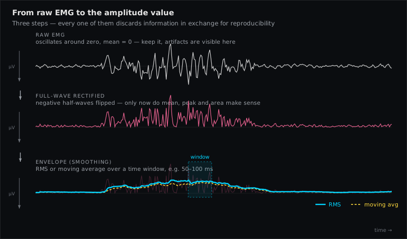
Step 1 — Full-wave rectification#

The raw EMG oscillates around zero; its mean is zero. Rectification flips every negative value to positive (full-wave) or discards it (half-wave; rarely used). Only after rectification do mean, peak and area make sense (Konrad, p. 26). Nothing else changes: the timing of every spike is preserved.

Step 2 — Smoothing: the envelope#

Smoothing averages the rectified signal over a moving window and produces the linear envelope — the amplitude course without the spikes. Two algorithms are standard (Konrad, p. 27):

• Moving average (MovAg / ARV). The mean of the rectified signal within the window. SENIAM calls it the "average rectified value", an estimator of amplitude behaviour related to the area under the epoch.
• Root mean square (RMS). Square, average, take the root. Reflects the mean power of the signal and is the recommended choice (SENIAM, De Luca). At the same window RMS gives somewhat higher values than the moving average — the two are not interchangeable in absolute terms, though the curve shape is almost identical.

Window length decides the trade-off between calm and timing. Konrad: 20 ms for fast events (jumps, reflexes) up to 500 ms for slow or static tasks; 50–100 ms works in most conditions. Longer windows smooth more but introduce a phase shift — the envelope lags behind steep onsets, which matters for timing analyses. Compare the Tibialis Anterior burst at heel strike (short window) with a sustained Longissimus Thoracis hold (long window is fine).

An alternative to the moving window is a low-pass filter — Konrad's example: a 2nd-order Butterworth at 6 Hz applied forwards and backwards (zero phase shift). It produces the same envelope shape and amplitude statistics as a ~100 ms moving average, without the lag.

Step 3 — Digital filtering: less is more#

Konrad, SENIAM and ISEK agree: with modern amplifiers, no additional filtering is needed in regular kinesiological EMG. The recommendation is the full 10–500 Hz band. Two specific warnings:

• No notch filter for 50/60 Hz. It removes real EMG power in the very region where the spectrum peaks. Solve mains hum at its cause — grounding, cable fixation, reference electrode (see the ten factors).
• A high-pass at 20–25 Hz is acceptable for fine-wire recordings and dynamic tasks with cable movement; it does not materially change ensemble-averaged gait curves. Any higher and you start cutting the fatigue-relevant low-frequency content.

Konrad adds a caution worth repeating: biofeedback units that display heavily pre-processed signals should not be used for scientific studies. For biofeedback itself the envelope is exactly what the user needs — as long as everyone knows it is an envelope.

From envelope to numbers#

The envelope is what amplitude parameters are computed from (Konrad, p. 39):

• Mean over an analysis interval — the most important and most robust value; least sensitive to interval length; best for comparisons.
• Peak — too variable on a single trial; meaningful for averaged curves. Konrad's compromise: average peak, the mean of e.g. the ten highest values in the interval.
• Area (integrated EMG, iEMG) — the integral, in µV·s; grows with interval length, so only comparable at equal durations. Historically "iEMG" was also used loosely for analog-smoothed curves.
• Input % — the mean of each channel expressed as a share of the summed means of all channels; a distribution analysis for comparing muscle ratios between exercises.

Which of these answers which question is the subject of EMG parameters — which question; making the numbers comparable across sessions and people is the subject of normalisation.

What to report#

ISEK's reporting standard and SENIAM ask for the complete chain, because two labs with different windows get different numbers from the same muscle:

1. Amplifier bandpass and sampling rate.
2. Rectification (full-wave).
3. Smoothing method (RMS / moving average / low-pass filter) and window length or cut-off frequency.
4. Any additional filter (type, order, cut-off, zero-phase or not).
5. Amplitude parameter (mean, RMS, peak, area) and analysis interval.
6. Normalisation method.

Keep the same chain for everything you compare — a reference contraction processed with a 300 ms window does not normalise a trial processed with 50 ms.